|
In this project, I implemented a pathtracer which renders images using global illumination. In order to do so, rays are casted from the camera through each pixel with the intent of locating an intersection point. We locate these intersections using the Moller Trombore algorithm for triangles, and the sphere intersection equation for spheres. To drastically improve the efficiency of this process, we implement a bounding volume hierarchy (BVH) to recursively split the bounding box into more managable subsets for intersection testing. Once we find the intersection point, we can cast sample rays to each light in the scene in order to generate direct lighting. We can then bounce these rays recursively to generate indirect lighting, allowing for global illumination. Finally, we improve the efficiency of the overall algorithm using adaptive sampling, which takes advantage of the fact that some pixels converge earlier than others.
Given the origin (x, y) of a pixel, a set number (ns_aa) of camera rays are generated and traced through the scene. For each sample, a random offset is generated using the gridsampler->get_sample() function. If the number of samples is one, however, the offset is set to be (0.5, 0.5). This offset is added to the origin point of the pixel. This point is then normalized to the appropriate range of [0, 1]^2 by dividing the x and y values by the pixel buffer width and height, respectively. This sample point then gets passed into generate_ray in camera.cpp. This function, which will be implemented in task 2, generates the appropriate ray, which is then passed into est_radiance_global_illumination. This function, as the name suggests, evaluates the rays radiance. This radiance is then stored in a spectrum. Every sample will produce a radiance value which will be added to this spectrum, which is then returned.
The Camera::generate_ray function is used in the previous part to get a ray from a given sample point. The bottom left and top right points are first calculated as
Vector3D(-tan(radians(hFov)*.5), -tan(radians(vFov)*.5),-1)
Vector3D( tan(radians(hFov)*.5),  tan(radians(vFov)*.5),-1)
We can then linearly interpolate these two points with the input point in order to scale the sample to the size of the sensor plane. We can then return Ray(pos, c2w * Vector3D(sx, sy, -1)), were sx and sy are the x and y values of the interpolated point. The c2w transform converts the vector to world space.
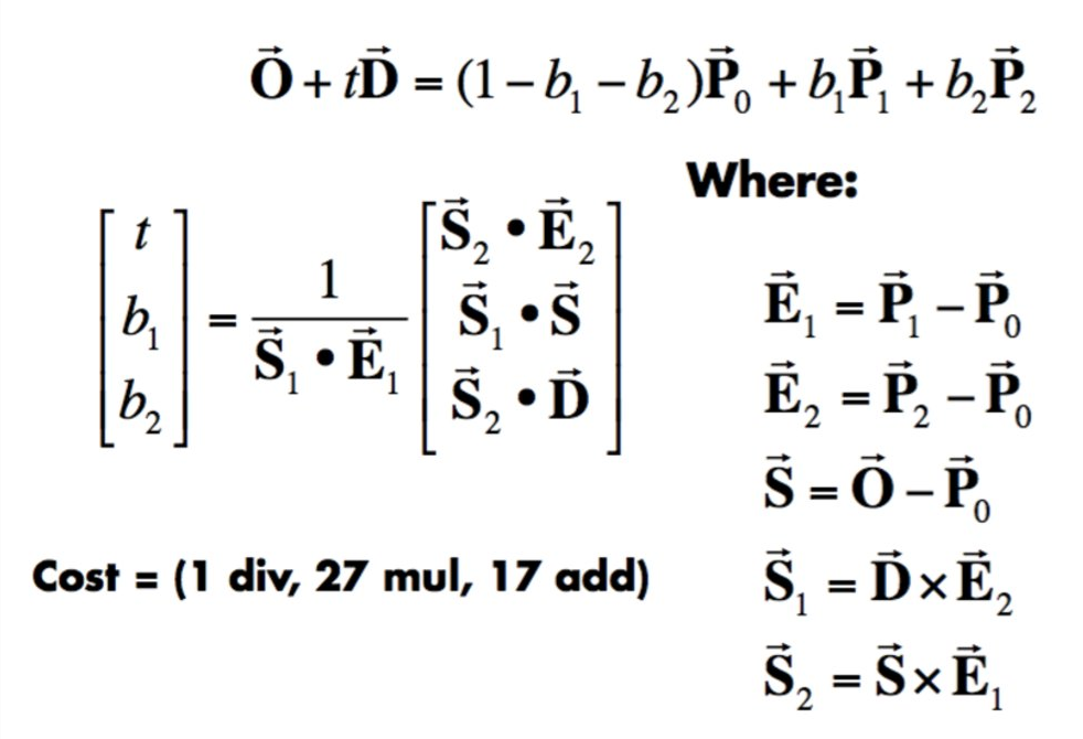
In this section, we implement ray-triangle intersection using the Moller Trumbore algorithm from lecture, pictured below.
|
|
We first define each of the variables specified in the algorithm. We can then use dot products to calculate the [t b1 b2] matrix. Now we have the t value, as well as the first two barycentric coordinates. As we know from project 1, we can calculate the third barycentric coordinate b3 as 1 - b1 - b2. If any of the barycentric corrdinates are outside the (0, 1) range, or if the t value is outside the (min_t, max_t) range of the given ray, we return false. Otherwise, we update the ray's max_t to the new t value, set the surface normal at the hit point as the interpolation between the barycentric coordinates and the per-vertex mesh normals, and return true.
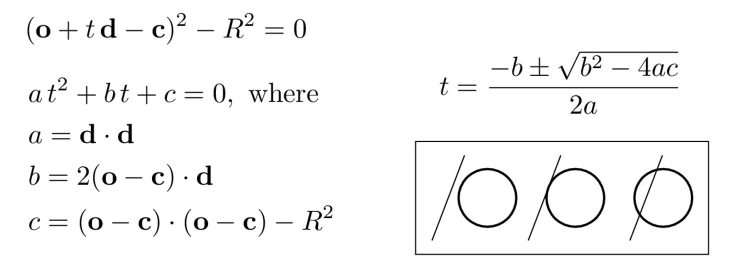
In this section, we implement sphere-triangle intersection using the quadratic formula. The relevant lecture slide is pictured below.
|
We first implement Sphere::test() as a helper function, defining the variables a, b, and c as specified in the algorithm. We can then calculate the determinant, and if it is negative we immediately return false. Then the quadratic formula is used to calculate t1 and t2. We return that these values are in the appropriate range (min_t, max_t) and that at least the larger of the two (t2) is nonnegative. Now we move on to the intersect functions. We call the test function; if it returns true, the new t value can be assigned to ray.max_t. If t1 > 0, t = t1, otherwise t = t2. We know t2 must be positive because of the check in the helper function. If there is an intersection argument (i), we normalize r.o + r.d * t - o and set that value as i->n.
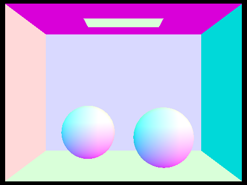
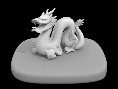
Now that al four tasks have been completed, the dae files can be rendered as images, although the process at this point is very slow. The final result can be seen below.
|
Below are some more renderings of smaller dae files that show the normal shading:
|
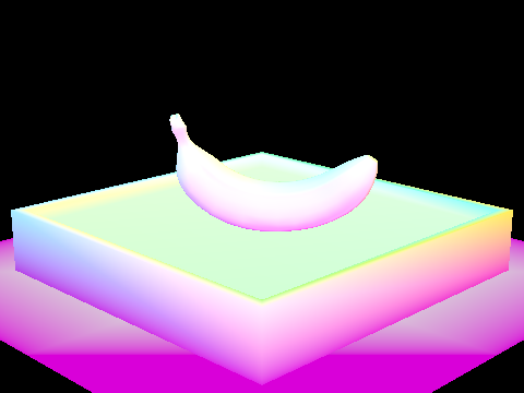
|
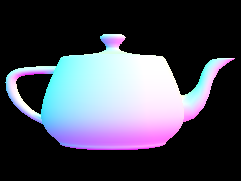
|
|
Larger dae files take a long time to complete. For instance, meshedit/cow.dae, takes 356.0654 seconds- nearly 6 minutes. Implementing BVH will result in a dramatic speedup. First, we compute the bounding box of the given primitives and initialize a new BVHNode with that bounding box. If there are <= max_leaf_size primitives, then the node is a leaf. In this case, we simply initialize the node's primitive list with the given primitives and return the node. Otherwise, we need to calculate the split point and recurse. We initialize two vectors of primitives, one for the left side and one for the right. Before we calculate the split point, we need to decide which axis we are splitting. Looking at the extent of the bounding box, the axis should be that of the largest dimension. Once we have this, we can calculate the split point as centroid_box.min[axis] + axis_len / 2, which is the midpoint of the bounding box on the chosen axis. Now we can loop through each primitive p, adding it to the left vector if p->get_bbox().centroid()[axis] < split, and to the right vector otherwise. We then recursively call the function on the left and right vectors until we have our root node. To prevent infinite recursion in the case that all primitives lie on one side of the split, if either side is an empty vector we can simply move one of the primitives from the non-empty side to the empty side and continue the process.
Next, we implement BBox::intersect() to find the interval of t values for which a given ray lies inside the box. To do so, we need to check the ray's intersection of each plane (xy, yz, xz). We can achieve this using a for loop over the range(0,3) and the given points min and max. For each i, if r.d[i] is nonzero, then we calculate min_t and max_t as (min[i] - r.o[i]) / r.d[i] and (max[i] - r.o[i]) / r.d[i]. As we loop through, we update our t0 and t1 values to achieve the appropriate range. t0 evaluates to the maximum of the smaller t values from each iteration, and t1 evaluates to the minimum of the larger t values from each iteration.
Next, we implement the BVHAccel::intersect() routines. If the ray does not intersect the bounding box of the node, we return false. If the node is a leaf, we loop through the primitives to check if there is a hit. In the function with no intersection parameter, we can return true if there is a hit. Otherwise, we simply set the boolean variable hit to true. Each time we test an intersection, we increment total_isects. If the node is not a leaf, then we recursively call intersect on the left and right vectors of the node. We then set hit to true if either of the recursive calls is true. I was initially placing both recursive calls on one line as intersect(ray, i, node->l) || intersect(ray, i, node->r). However, this results in shortcircuiting. If the left recursive call returns true, intersect(ray, i, node->r) will never be called. To fix this, I simply put each recursive call on it's own line and set hit = left || right afterwards.
All of my code seemed correct to me, however, I kept getting partial renders. It was as if only the leftmost leaf node was being rendered. If I switched the order of the recursive calls, only the rightmost leaf node would be rendered. Here is a screenshot of the single rendered leftmost leaf node.

|
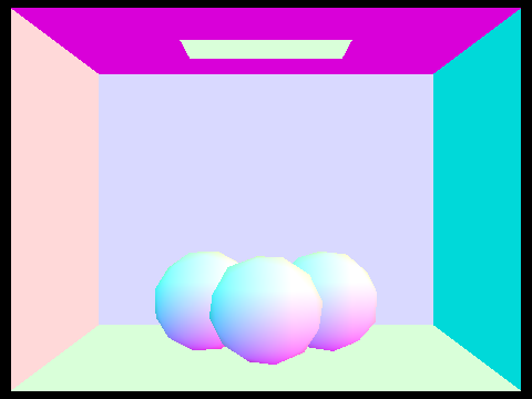
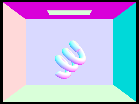
It turns out, the reason for this was my intial call to node->bb.intersect(). I was calling node->bb.intersect(ray, min_t, max_t) as opposed to setting variables t0 and t1 as min_t and max_t and calling node->bb.intersect(ray, t0, t1). This was mutating the min_t and max_t values, resulting in the partial renders. Once I fixed this error, everything worked as expected. Rendering the dae files now took a fraction of the original time, so large files were no longer a problem. Here are some larger dae files rendered:
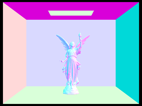
|
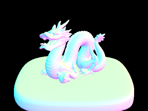
|
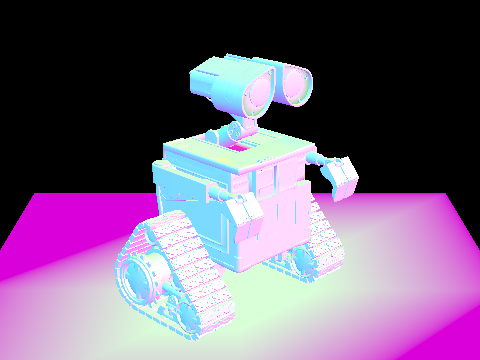
|
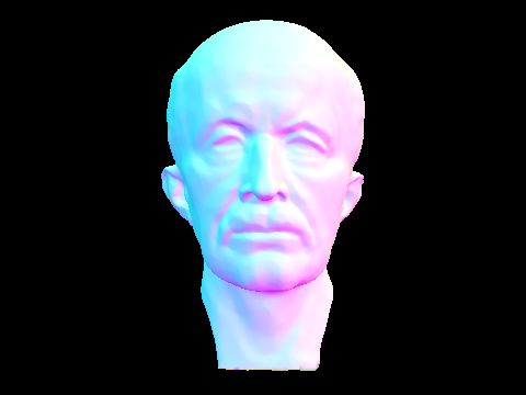
|
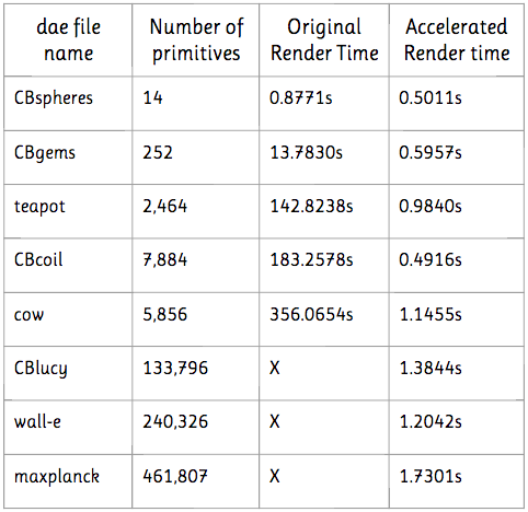
The speedup was quite dramatic, and I documented some of the results in the table below. I did not attempt to render any of the large dae files before implementing BVH acceleration, as it would have taken too long and my laptop is an old man who is just trying his best.
|
The smallest file (CBspheres) showed little speedup, as can be expected. However, the second smallest file (CBgems), already demonstrated a 23x speedup. teapot.dae rendered 146 times faster, CBcoil.dae 366 times faster, and cow.dae 310 times faster. wall-e.dae is over 40 times larger than cow.dae and yet they render in almost the same time. Essentially, BVH acceleration has allowed us to avoid the approximately linear increase in render time that we were experiencing before. Now, all the files render in approximately the same time (2 seconds, max), regardless of size.
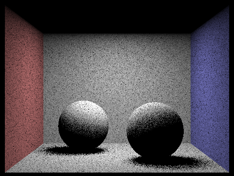
In this part, I implemented two methods of direct lighting: uniform hemisphere sampling and importance sampling. Note that the rendered images in this part do not contain the direct light source, as that will be implemented in part 4.
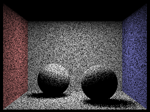
Uniform hemisphere sampling take samples in a uniform hemisphere around a hit point. For each ray that intersects a light source, the incoming radiance from that light source is calculated, converted to outgoing radiance, and averaged across all samples. First, we define the pdf as 1 / 2 * PI. In a loop, we take num_samples samples using hemisphereSampler->get_sample(). This function returns the direction of the ray in object space, which we need to transform to world space using the matrix o2w. Next, we cast a ray from the hit point in the direction of the sample (wi_world). When initializing the ray, we must offset the origin by EPS_D * wi_world to avoid floating point imprecision errors. We also create a new intersection isect2 and check for an intersection using bvh->intersect(ray, &isect2). The information from the intersection will now be stored in isect2. If there is an intersection, then we increment the total outgoing light L_out by isect2.bsdf->get_emission(), scaled by the BSDF and the cosine term. Once we have collected all samples, we average L_out by dividing by num_samples * pdf. At first I was getting completely black renders, when my code seemed to be correct. This was actually caused by an error in my triangle intersection function, where I accidentally deleted the line which assigned a t value to the intersection. Once I added this line back in, my renders came out as expected. The images below have been rendered using uniform hemisphere sampling.
|
|
|
|
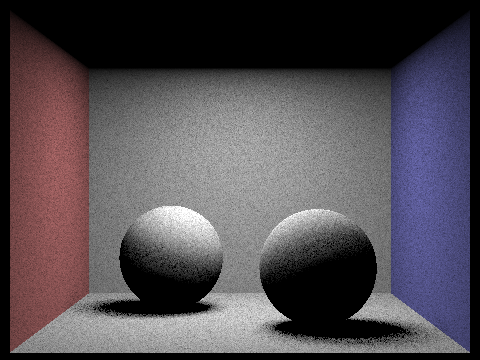
Uniform hemisphere sampling results in a lot of noise. To avoid this, we can implement importance sampling: instead of uniformly sampling in a hemisphere, we sample each light directly. For each light in scene->lights, we first need to determine the number of samples. If the light is a delta light, we only need one sample. Otherwise, we need to take ns_area_light samples. For each sample we calculate L_in as light->sample_L(hit_p). This function also sets the values for wi (the direction from hit_p to the light source), distToLight (the distance from hit_p to the light source), and the pdf (evaluated at wi). The direction wi is in world space. In order to pass it to the BSDF we need to convert it to object space as w_in = w2o * wi. Next, we check if the z coordinate of w_in is 0, which means the light point lies behind the surface. If this is th case, we can continue the loop. Otherwise, we will cast a shadow ray with origin EPS_D * wi + hit_p, direction wi, and max_t distToLight. As in uniform hemisphere sampling, we need to offset the origin to avoid floating point imprecision errors. We set max_t to distToLight to make sure we are not checking intersections behind the light source. If the ray does not intersect the scene, then we increment L_out by L_in * isect.bsdf->f(w_out, w_in). Again, we must scale by the cosine term and divide by the pdf. For each light, we must also average by the number of samples. The images below have been rendered using importance sampling.
|

|
|
|
The images below are rendered using increasing numbers of samples per area light and one camera ray per pixel (s = 1)
|
|
|

|
We can see the noise decrease and the shadows become smoother and more natural as the number of samples per area light increases.
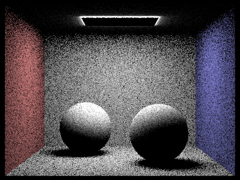
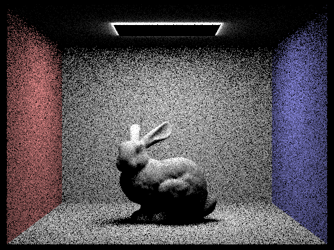
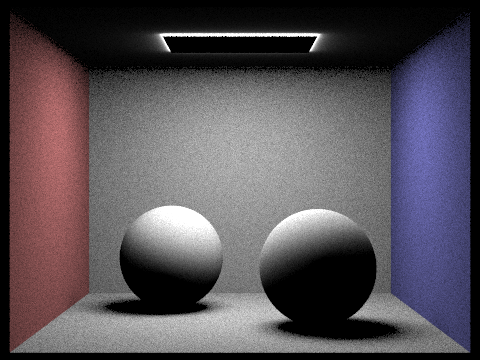
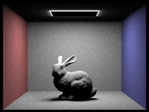
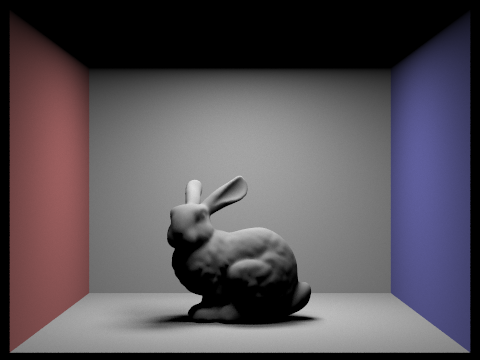
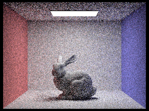
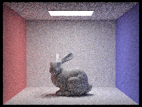
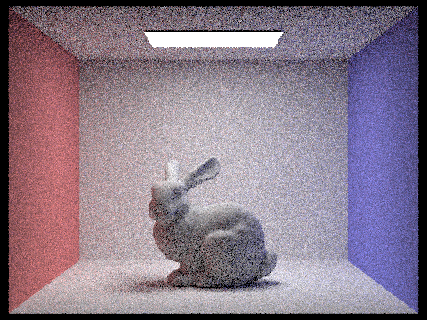
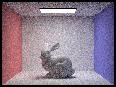
The below images show CBbunny rendered using uniform hemisphere sampling and importance sampling at two settings.
|
|
|
|
|
|
The difference between the two methods is quite drastic, and anyone can see that importance sampling results in far less noise than uniform hemisphere sampling. In uniform hemisphere sampling, lower sampling rates produce a lot of noise, but this is significantly reduced by upsampling. However, this means that it takes a very long time to render a less noisy image, as we have to perform 4 times as many samples. With importance sampling, there is little noise even at a low sampling rate. In fact, the image rendered using importance sampling at a low sampling rate has less noise than the image rendered using uniform hemisphere sampling at a high sampling rate. This means that we can produce images with minimal noise levels much more efficiently, with far fewer samples. Using importance sampling at a high sampling rate results in almost no visible noise! Overall, in terms of time and efficiency, it is much more worthwile to use importance sampling over uniform hemisphere sampling.
The next step is implementing indirect lighting to allow for global illumination. We do so using the rRussian roulette termination technique. If the max depth is 0, we return Spectrum(0,0,0), since we will not need to determine direct or indirect lighting. If the max depth is 1, we only need to determine direct lighting. When the max depth is greater than 1, we need to calculate the indirect lighting. First we need to set the probability of not terminating the ray (cpdf), which I set as 0.7. Using the coin_flip function, if (coin_flip(cpdf) || (r.depth == max_ray_depth)), we do not terminate the ray. Since r.depth is initialized to max_ray_depth, If r.depth == max_ray_depth, then this is the first iteration of sampling for indirect lighting. Since at this point we know max_ray_depth > 1, we still need to perform at least one level of indirect light sampling. This is why we include this condition in the if statement.
Now we need to actually start sampling. We declare the bsdf sample as isect.bsdf->sample_f(w_out, &w_in, &pdf). This function, which we defined in the previous part, also sets the proper values for w_in and pdf to use later on in the function. The direction w_in is in object space, so we convert it to world space as wi = o2w * w_in (as in hemisphere sampling). Now we can declare a ray in this direction, with origin EPS_D * wi + hit_p. We set this ray's depth to the previous ray's depth - 1, to make sure that max_ray_depth is enforced. As in hemisphere sampling, we initialize a new intersection, isect2, to feed into bvh->intersect(bounced_ray, &isect2). The information is now stored in this new intersection. If there is a hit, then we need to pdate L_out. Define L_in as the recursive call, at_least_one_bounce_radiance(bounced_ray, isect2). Now we increment L_out by this amount, scaled by the bsdf sample and cosine term and divided by the pdf and cpdf. The shadows in my renders were initially turning out too dark, as shown below, and the overall image seemed a little dim.
|
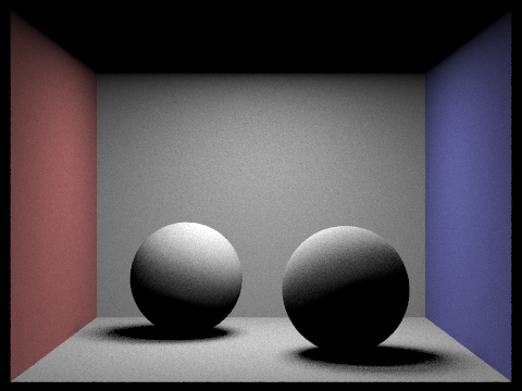
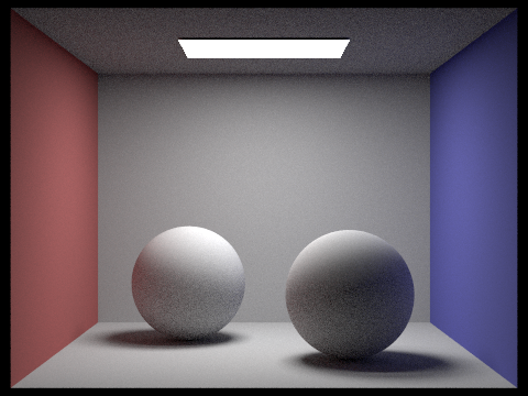
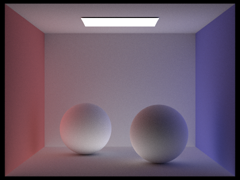
It turns out this was because I was multiplying by the bsdf twice, meaning the indirect bounces of light were not counting as much as they should have been. Once I fixed this, my renders matched the sample ones in the spec. The images below demonstrate the effect of adding indirect lighting. The light now bounces off of the surfaces, illuminating the room (hence the term "global illumination").
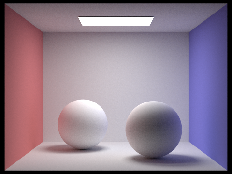
|

|
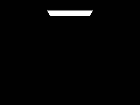
In the images below, we can observe the difference between direct and indirect lighting.
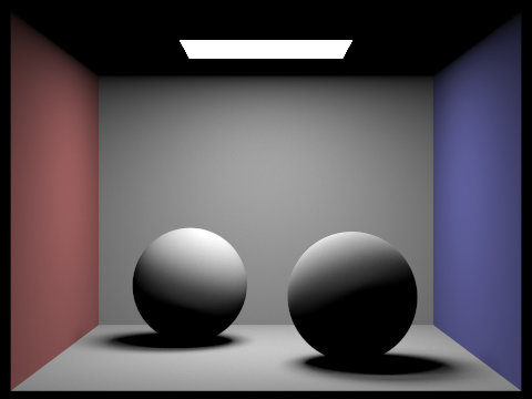
|
|
With direct lighting, only points that have a direct path to the light are illuminated. This means a lot of the image is very dark, which obviously is not how light works in the real world. Indirect lighting on its own is more muted and distributed around the scene. This is because all of the light has been bounced at least once, which means the brightness is not as intense.
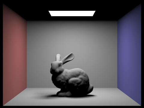
The images below show the effects of increasing the max ray depth. These images are rendered with the settings s=1024 and l=4.
|
|

|

|
With m=0, there are zero bounces, which means we only see light directly emitted to the camera. With m=1, there is only one bounce, which means we only consider direct lighting (as in the previous part). Once we increase m to 2, we start to see a difference, since we are now starting to add in some indirect lighting. The ceiling is now visible, as well as the bottom half of the bunny. As the max ray depth increases, the scene gradually becomes more illuminated. If we increase the max ray depth all the way to 100, the difference is very subtle, indicating that the values may have converged.

|
The images below show the effects of increasing the sample per pixel rate. These images are rendered with the settings l=4 and m=5.
|
|
|
|

|

|
At a low sample rate, there is a lot of noise in the rendered image, as expected. As we increase the sample rate, the noise decreases. This is because the image converges as the sample rate increases. If we increase the sample per pixel rate to 1024, there is essentially no visible noise in the rendered image.
|
|
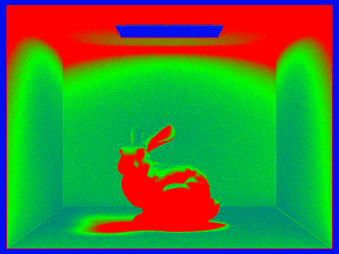
When rendering an image, some pixels converge faster with low sampling rates, while other pixels require a high number samples to eliminate noise. We can use this fact to increase the efficiency of our pathtracer with adaptive sampling. In our raytrace pixel function, we will keep track of two variables: s1, the sum of the sample illuminances, and s2, the sum of the squares of the sample illuminances. We can use these values to calculate the mean and variance at the current step, and then in turn use the mean and variance to determine whether or not the pixel has converged. If so, we can stop sampling. We define I as 1.96 * sqrt(variance) / sqrt(n). If I < maxTolerance * mean, then we can break from the loop. To keep the cost of the function from getting too high, we only perform this check every samplesPerBatch samples. Finally, we fill in the number of samples used for that pixel in the sampleCountBuffer vector, to produce sampling rate visualization images. I was initially getting an error where every pixel was taking between 450 and 600 samples, making the entire sample rate image appear in varying shades of teal, as pictured below.

|

|
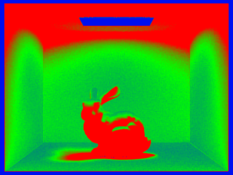
This turned out to be because I was accidentally using the total illuminance thus far at each iteration, as opposed to the illuminance of that specific sample. Once I fixed this, my sampling rate images started showing up properly.

|
|
However, I noticed some subtle differences between my sampling rate image and the staff's. For instance, I had more green pixels on the ceiling, and the bunny's shadow had slightly fewer red pixels around the edges. As an experiment, I changed my non-termination rate in my russian roulette from 0.7 to 0.6. This resulted in a similar sampling image with less green on the ceiling, but more green on the walls. These images are shown below.

|
|
The staff results seem to fall somewhere beteen these two, and the difference between the sampling rates could be due to some very minor difference in code. Regardless of this, the adaptive sampling works, allowing for an increase in efficiency when rendering images with a high sample rate.