|
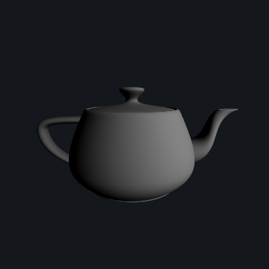
In this project, I extended my pathtracer to include different materials, lighting sources, and camera lenses. I also worked in GLSL to create several shaders which can be viewed in real time. I first implemented mirror and glass materials by incorporating reflection and refraction of light rays. I then moved on to microfacet material, to create the apprearance of metallic surfaces. This effect is achieved using reflection on isotropic rough conductors. In terms of lighting, I added a new type of light source- an infinite environment light. Environment lights supply incident radiance from all directions, and the source is thought of as being infinitely far away. This allows us to achieve lighting conditions which are more representative of the real world. Now, if a ray does not intersect with the scene, we sample light from the environment light. I also added a new type of camera lens, a thin lens. This allows us to incorporate field of view and focus/blur effects. Finally, I used GLSL to inplement several OpenGL shaders, including diffuse, Blinn-Phong, bump mapping, displacement mapping, and a few other custom shaders.
First we need to alter at_least_one_bounce_radiance() so it can handle non-diffuse materials. We only add one_bounce_radiance() to L_out if the current intersection is not a delta intersection. We must also check for delta intersections when there is an intersection with our bounced ray. If the current intersection is a delta intersection, we will add the zero_bounce_radiance() from the second intersection to L_in, in addition to the scaled recursive call.
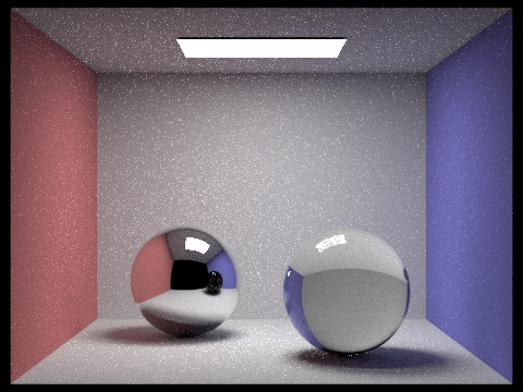
Next we implement the BSDF:reflect() function. This function reflects wo about the normal, (0,0,1), and then stores it in wi. We call this function in MirrorBSDF::sample_f() to set wi. We then set the pdf to 1 and return reflectance / abs_cos_theta(*wi). Now we can render mirror materials, as shown below (s=1024, l=4, m=5).
|
|
In order to render glass, we need to implement refraction using Snell's law. First we need to set our eta value, which depends on whether we are entering or exiting the material. When we are entering, wo.z > 0 and eta = 1 / ior, the index of refraction. Similarly, if we are exiting, wo.z < 0 and eta = ior / 1 = ior. From Snell's law, we calculate cosθ′ as 1 - (eta * eta) * (1 - (wo.z * wo.z)). If this value is less than zero, then we have total internal reflection, which means this function can return false. Otherwise, we convert our spherical coordinates phi and theta to cartesian ones. So wi.x = -eta * wo.x, wi.y = -eta * wo.y, and wi.z = -+sqrt(cosθ′). The sign of wi.z depends on whether we are entering or exiting, so intuitively it should have the opposite sign of wo.z.
Now we will use the Fresnel equations and Schlick's approximation to model the ratio of reflection energy to refraction energy, so we can render realistic glass material. If there is total internal reflection, we do the same thing as in MirrorBSDF::sample_f(). Otherwise, we need to calculate Schlick's coefficient, R, as shown below.
|
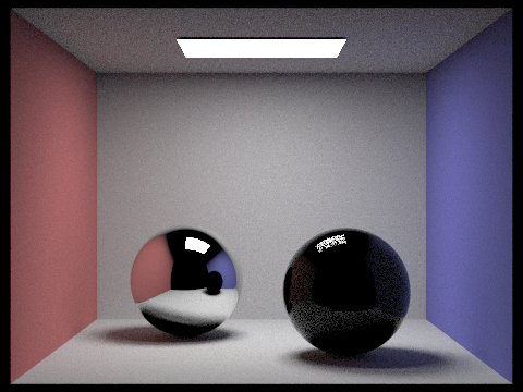
We use this term to determine whether to reflect or refract. If coin_flip(R), then we reflect. We set the pdf to R and return R * reflectance / abs_cos_theta(*wi). Otherwise, we refract. In this case, we set the pdf to 1 - R and return (1 - R) * transmittance / abs_cos_theta(*wi) / eta ^ 2, where eta is calculated the same way as in the refraction function. I was originally getting a lot of noise, but I was able to minimize this by changing my russian roulette non-termination policy to 0.9. Now we can render glass objects, like the one below (s=1024, l=4, m=5).
|
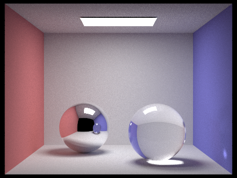
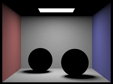
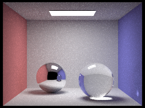
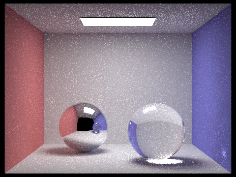
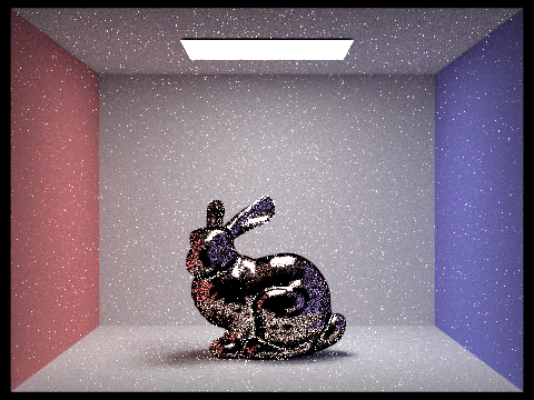
The image below shows two spheres, one made of mirror material and one made of glass (s=1024, l=4, m=5).
|
We can examine how the light reflects around the scene by changing the max depth. The following images have been rendered with 64 samples per pixel and 4 samples per light.
|
|
|
|

|
|
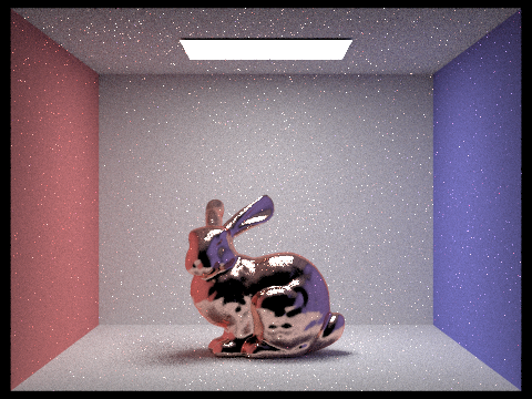
With a max depth of zero, we only see direct light emmissions. Once we increase the max depth to 1, we can see some direct lighting, but the spheres are still black. With m=2, the spheres finally start to reflect the light. In the mirror sphere we can see the reflection of the previous scene, with m=1. The glass sphere reflects some light too, but only a fraction of the rays are being reflected. The other rays intersecting with the glass sphere are being refracted, but we cannot see them yet because the rays are terminating before they can leave the sphere. We can see these refracted rays when m=3. At this point, the shadows on the mirror sphere are being illuminated as well. When we increase max depth to 4, the light leaving the sphere hits the ground, creating a caustic below it. Additionally, the glass sphere is now reflected in the mirror one, appearing as blue instead of black. There is also a small bright spot on the bottom right side of the glass sphere. When m=5, this bright spot is reflected onto the blue wall. If we use a max depth of 100, Russian roulette will terminate the rays, producing a slightly brighter but similar image to that of max depth = 5.
|
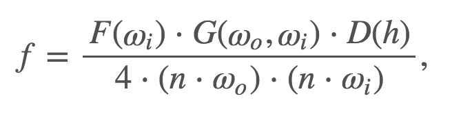
The microfacet model allows us to render metallic materials. The first step is implementing the BRDF evaluation function, MicrofacetBSDF::f(). This step is quite straightforward, as we simply want to call the various elements in the following equation:
|
where F is the Fresnel term, G is the shadowing-masking term, and D is the normal distribution function (NDF). We will implement the F() and D() functions next.
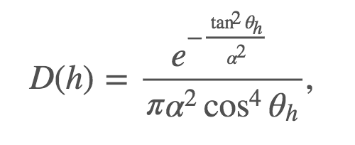
The NDF defines how the microfacets' normals are distributed. From the spec, we will use the Beckmann distribution to calculate the NDF:
|
where α is the roughness of the macro surface, θh is the angle between h and the macro surface normal n.
Next, we need to calculate the fresnal term. We cannot use Schlick's approximation, since that is for air dialectric interfaces, and microfacet materials are air conductors. From the spec, we will use the following approximation to calculate F:
|
where η and k are used together to represent indices of refraction for conductors.
At this point, we can render microfacet materials using cosine sampling. However, we can drastically improve this in terms of noise level and efficiency using importance sampling. First, we get a sample point uniformly distributed within [0,1). We use this sample point, r, to calculate θh and ϕh, as shown below.
|
We can convert θh and ϕh from spherical to cartesian coordinates to get the vector h. Now we can calculate wi by reflecting wo over h as -wo + (2 * h * dot(wo, h)). If wi.z < 0, then we can set the pdf to zero return an empty Spectrum. If wi.z >= 0, then we can proceed to calculate the pdf. First, we can use our θh and ϕh to calculate pθ and pϕ as shown below.
|
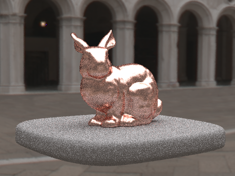
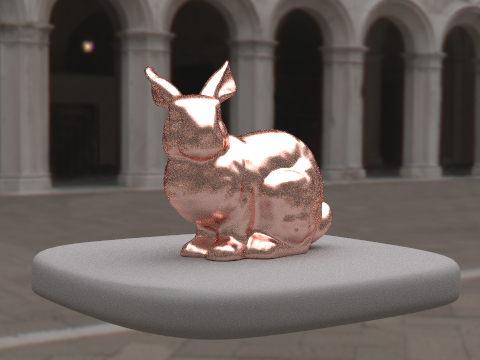
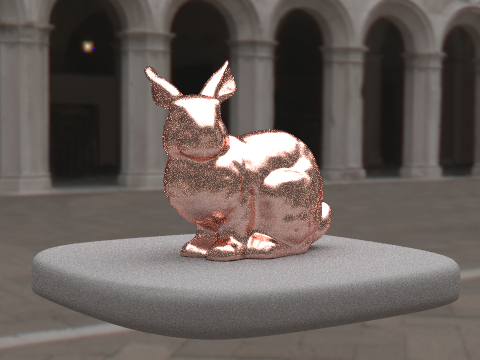
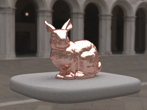
With these value, we can calculate p(h) as (pθ * pϕ) / sin(θh). Finally, we set our pdf to p(wi) = p(h) / 4(wi⋅h) and return the sampled BRDF value. I was originally getting a white outline around my bunny, which was caused by not checking for invalid samples in at_least_one_bounce_radiance (when pdf = 0). Once, I added this check, the white outline went away. With importance sampling, we can render microfacet materials with much less noise. Here are some renders demonstrating the microfacet materials copper and gold (s=1024, l=4, m=5).

|
|
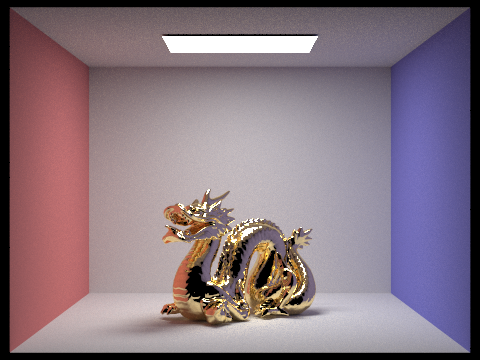
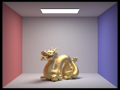
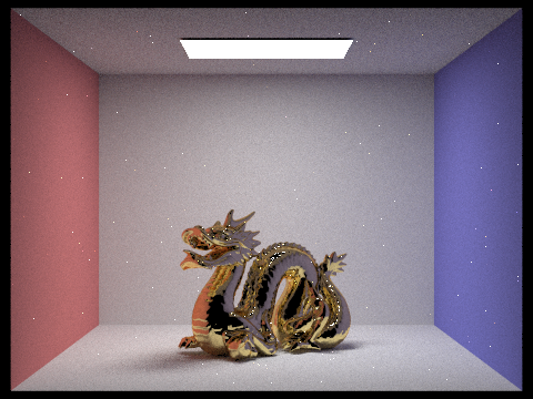
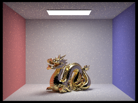
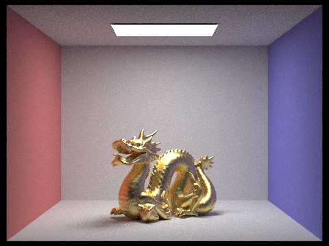
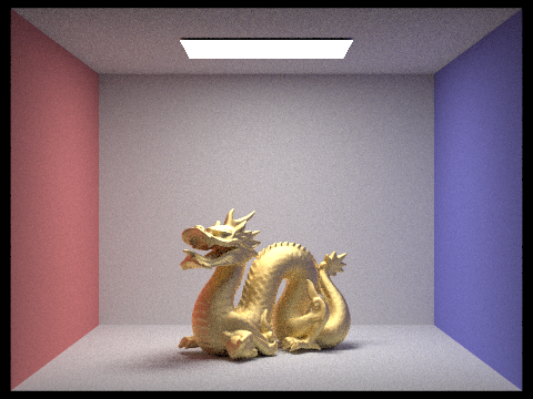
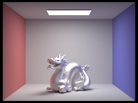
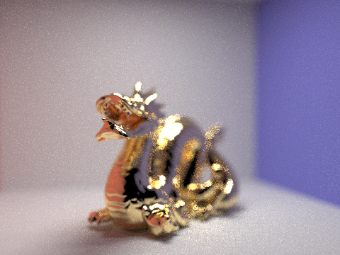
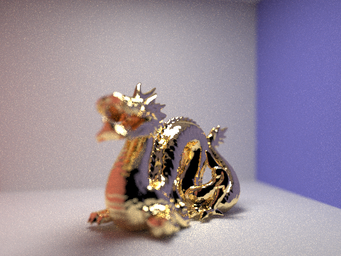
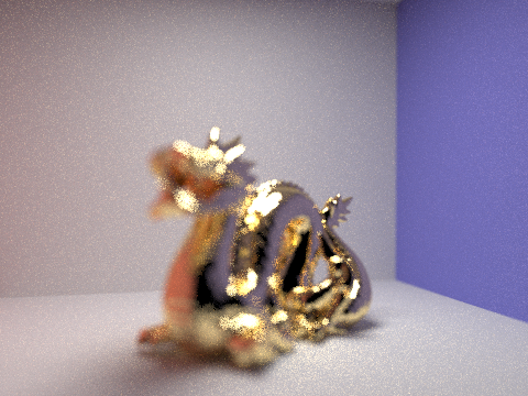
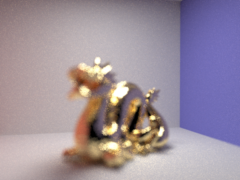
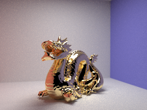
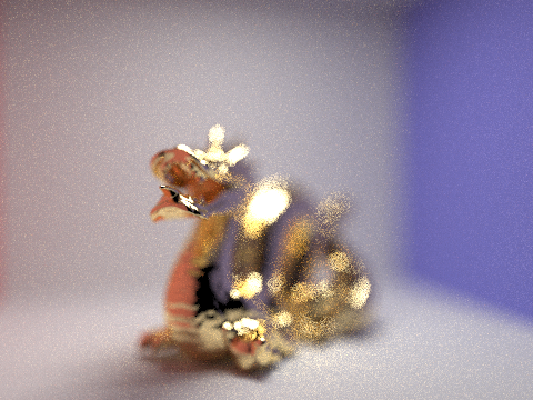
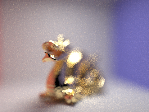
We can change the alpha value of a material to change how shiny or matte it appears. As the alpha value increases, the dragon becomes more matte. The renders below show what the dragon looks like with different alpha settings (s=128, l=1, m=5).
|
|
|
|
There is quite a difference in our renders when using cosine hemisphere sampling compared to importance sampling. While both techniques are correct, cosine hemisphere sampling takes a very long time to converge. We would need to use a very high sampling rate to get a decent image. Importance sampling, on the other hand, can render a much better image with far fewer samples per pixel. When we compare images rendered at the same settings (s=64, l=1, m=5) using both methods, the difference is clear. Cosine hemisphere sampling produces a lot of noise, and the bunny appears very dark and spotty. With importance sampling, there is less noise and the bunny is much more filled in, with a smooth, metallic look.
|
|
We can also alter the eta and k values at the wavelengths associated with red, green and blue to easily change the material of an object. I changed the dragon's material to silver and bronze in the images below. (s=1024, l=4, m=5).
|

|
First we need to update estimate_global_radiance() to get the environment map to appear. If there is no intersection and there is an environment map, then we return envLight->sample_dir(r). Otherwise we return an empty spectrum, as before. In at_least_one_bounce_radiance(), we also need to account for this. Again, if there is no intersection and there is an environment map, we call sample_dir(r). We take this as our sampled radiance, scale it by the appropriate factors, and add it to L_out. For uniform sampling, all we have to do now is set wi to a sample direction using sampler_uniform_sphere, convert this direction to (ϕ,θ) and then (x,y) coordinates, and use this look up the appropriate radiance value in the texture map using bilinear interpolation. We also set the pdf to 1 / 4π and the distToLight to INF_D.
We can improve the noise level by implementing importance sampling. First we need to calculate the necessary probabilities, given the pdf_envMap data. We normalize this data by dividing by the total sum. We then loop through for j = 0 to height and i = 0 to width to calculate the marginal and conditional probablitlies. We keep track of two values when calculating these values: the ongoing sum of pdf values and the sum of pdf values for the current height value. We fill in marginal_y using the former and conds_y using the latter.
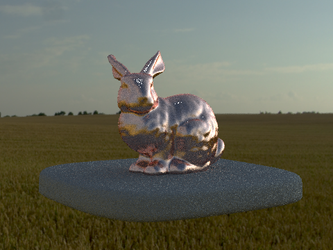
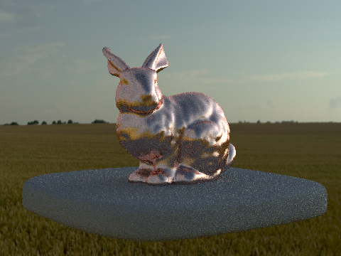
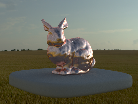
Now that we have these values, we generate a sample using sampler_uniform2d.get_sample(). We then use the inversion method to calculate our x and y values. std::upper_bound allows us to calculate the index of the first y value in marginal_y that is larger than sample.y. Then we can use upper_bound to calculate the index of the first x value in conds_y (with the calculated y value) that is larger than sample.x. We use these x and y values to calculate the direction wi. We set distToLight to INF_D and pdf to (pdf_envmap[w * y + x] * w * h) / 2π^2 sin(θ). Then we return envMap->data[w * y + x]. When I rendered the copper bunny with the field environment, I noticed some strange white spots showing up. These spots were not present with the other exr files.
|
It took a while to track down what was going wrong, but it turned out to be a floating point error. Essentially, the y value of wi in at_least_one_bounce_radiance() was being set as 1.0028 instead of 1. Since wi is the direction of the ray we call sample_dir() on when there is an environment light, it gets fed into dir_to_theta_phi(). However, in this function, we take acos(dir.y). This means we are taking acos(1.0028), which returns nan. The staff code has dir.unit() as the first line in this function, but this does not actually change anything, since it is not altering the values. I originally fixed the issue by simply adding a check in at_last_one_bounce_radiance(), After adding this, the white spots went away but my renders still seemed a little noisy. These renders use importance sampling and are with 4 samples per pixel, 256 samples per light, and a max ray depth of 5.
|
|
Both the white spots and the noise actually stemmed from not normalizing the ray direction in Camera::generate_ray(). Once I added this, the white spots went away and the noise at the base cleared up. The images below have been rendered using importance sampling with the same settings as above (s=4 l=256 m=5).
|
|
And here's some with 256 samples per light, 16 samples per pixel, and a max ray depth of 5.

|

|
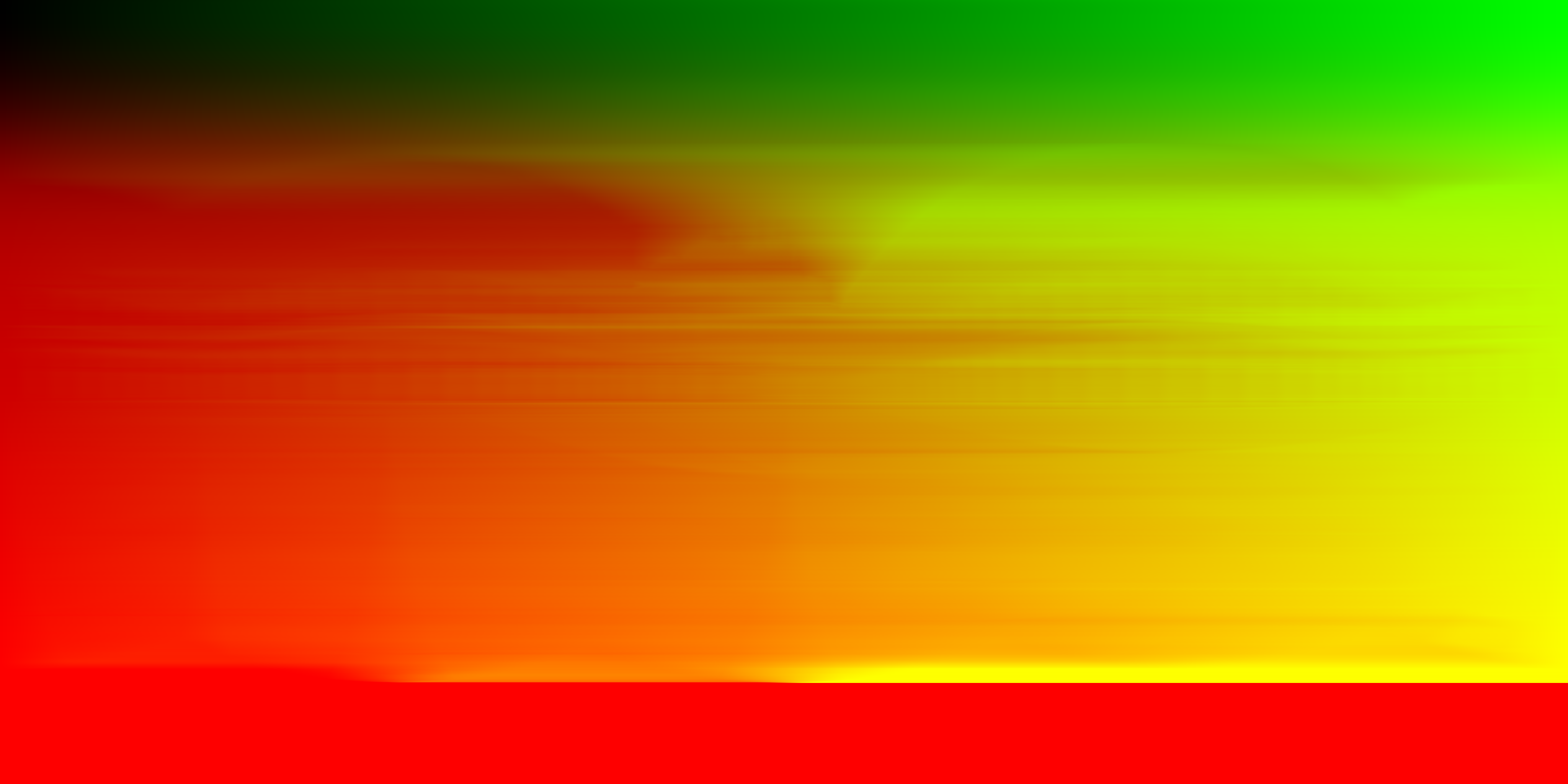
The following images have been rendered using the environment map and corresponding probability distribution pictured below.
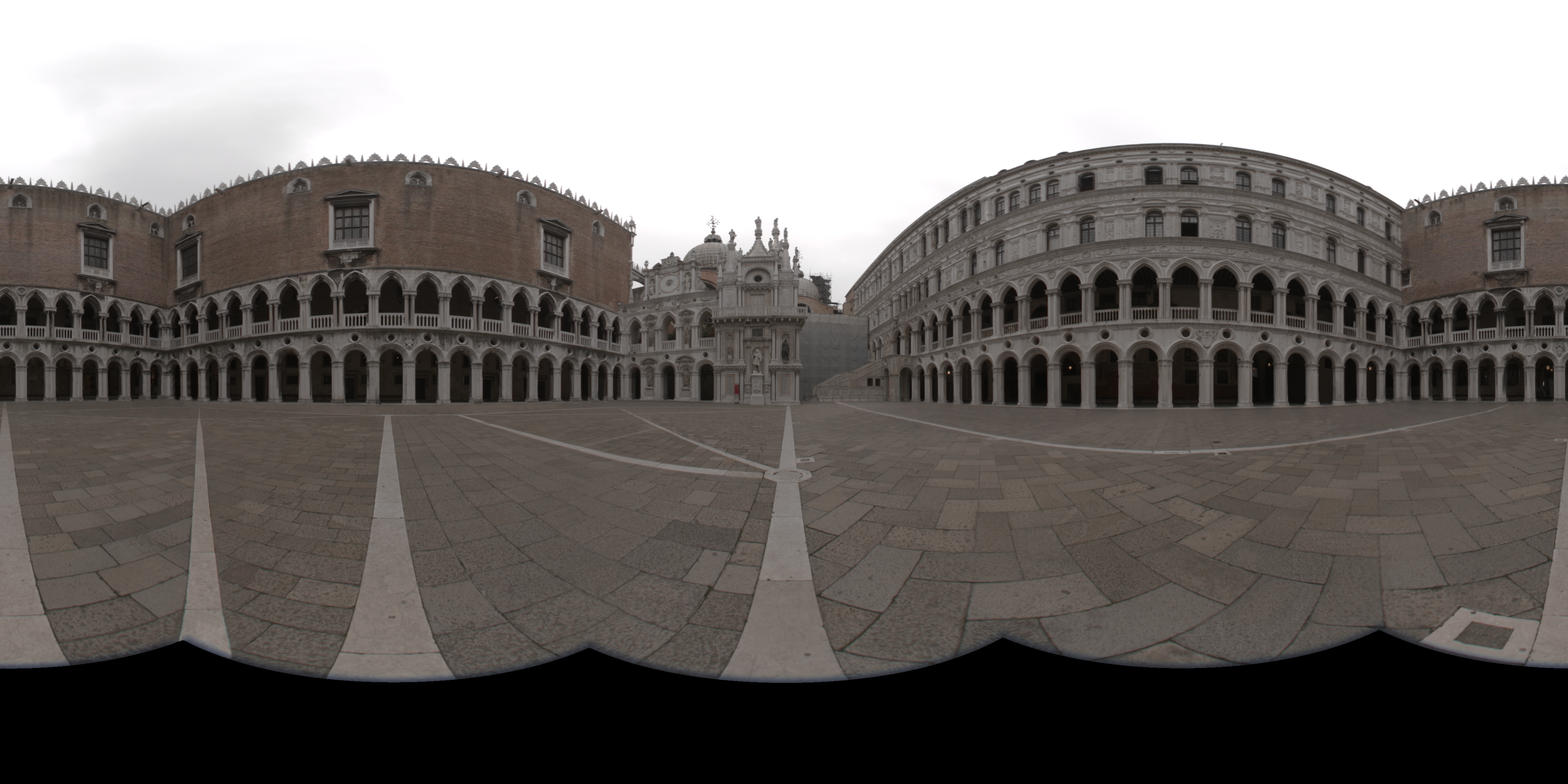
|
|
In bunny_unlit.dae, the bunny is made of diffuse material. The difference between uniform and importance sampling is not very noticable, but the latter has slightly less noise. These renders have been generated with 4 samples per pixel and 64 samples per light.
|
|
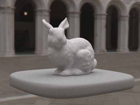
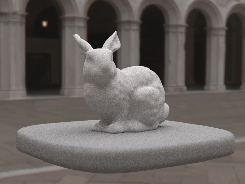
In bunny_cu_unlit.dae, the bunny is made of microfacet copper material. With uniform sampling we can see slightly more noise on the bunny, particularly around the right side of its face/chest. Again, the differnce is very subtle. These renders have also been generated with 4 samples per pixel and 64 samples per light.
|
|
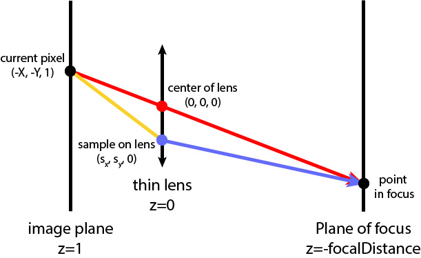
We can simulate a thin lens to enable depth of field. From the image below, the red ray is the one we implemented in project 3-1, and the blue ray is the one we will implement now.
|
First we get the direction of our original ray from project 3-1 part 1. We create a ray (the red ray) with this direction and origin (0,0,0). Next, we sample the thin lens disk uniformly as pLens=(lensRadius * sqrt(rndR) * cos(2π * rndTheta), lensRadius * sqrt(rndR) * sin(2π * rndTheta),0), where rndR and rndTheta are random numbers uniformly distributed in [0,1). Next, we calculate pFocus as the intersection between the red ray and the plane of focus (at z = -focalDistance). The blue ray is the ray that originates at pLens and points toward pFocus, meaning its direction is pfocus - plens. We normalize the direction, perform camera-to-world conversions on both the origin and direction, and add the camera's position to the origin. Now we can render images with depth of field. The image below was rendered with 256 samples per pixel, 4 samples per light, max ray depth 8, lens radius 0.0883883, and focal distance 1.7.
|
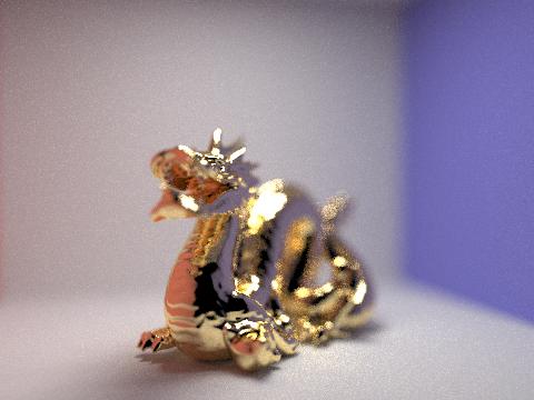
The images below have been focused at different depths. Smaller focal distances focus closer to the camera, while larger focal distances focus further back in the scene. With d=1.5, the dragon's head is the focus, while with d=3.0, the back wall is the focus. The other images fall somewhere in between, focusing on the dragon's body or tail. All images have been rendered with 128 samples per pixel, 4 samples per light, and max ray depth 8.
|
|
|
|
These images have been rendered with different lens radius values, but all are focusing on the same part of the image (the dragon's mouth). A smaller lens radius correlates to a larger range of focus in the image. All images have again been rendered with 128 samples per pixel, 4 samples per light, and max ray depth 8.
|
|
|
|
In this section we will use GLSL to implement shaders that can be rendered in real time. We use two OpenGL shader types to do so- vertex shaders and fragment shaders. Vertex shaders, as the name suggests, transform the vertices in our mesh, changing their position and normal values to generate different effects. The final position is written into gl_Position, which is the global position of the vertex. The output of the vertex shader is given as the input to the fragment shader. In the fragment shader, the geometry given by the vertex shader is broken down into fragments. The fragment shader computes a color for the given fragment, and writes this value into gl_FragColor. All of the GLSL shaders I have implemented and described below can be seen here.
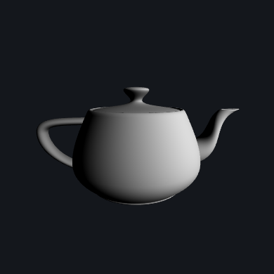
First we will implement the most basic shading- diffuse. In diffuse.vert we set fPosition and fNormal to the position and normal in screen space, and gl_Position to the position in global space. In diffuse.frag, we return the color of the fragment as Ld = kd * (I/r^2) * max(0, n⋅l). Here are the results of diffuse shading on the Utah teapot model.
|
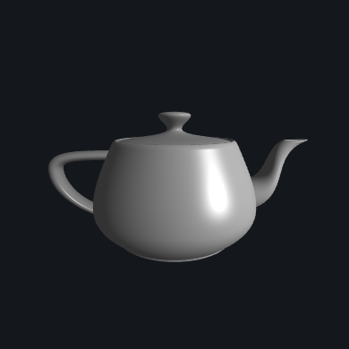
Next we implement Blinn-Phong shading to allow for specular lighting. In Blinn-Phong, we are now taking into consideration the ambient and specular lighting, in addition to diffuse lighting. These three components work together to create a more realistic effect. We calculate diffuse lighting as in the previous part. For specular lighting, we calculate the half vector h and choose an exponent p. Ls can then be calculated as ks * (I/r^2) * max(0, n⋅h)^p, where ks is the specular coefficient. Overall, the total lighting can now be described as:
L = ka * Ia + kd * (I/r^2) * max(0, n⋅l) + ks * (I/r^2) * max(0, n⋅h)^p
The images below demonostrate the effect each lighting component has on the final outcome. Ambient lighting is the base level lighting, diffuse lighting is the same as the previous part, and specular lighting adds a highlight to give the object some shine. The k coefficients and p can be adjusted to change the final appearance, but the settings for these images are ka=0.2, kd=0.6, ks=0.6, p=100.

|
|

|
|
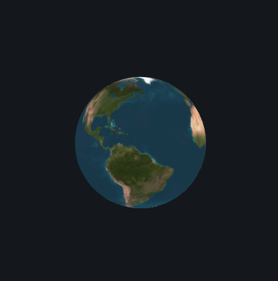
We can use the built in function texture2D(sampler2D tex, vec2 uv) to map a texture to an object. The image below is of a sphere with a texture image of Earth. Just like project 1, but now in 3D.
|
In order to add 3-dimensional texture to our objects, we use displacement and bump mapping. For bump mapping, we return fPosition and gl_Position as before, but we alter fNormal. We first calculate dU and dV as
dU = (h(u + 1/w, v) − h(u, v)) ∗ kh ∗ kn
dV = (h(u, v + 1/h) − h(u, v)) ∗ kh ∗ kn
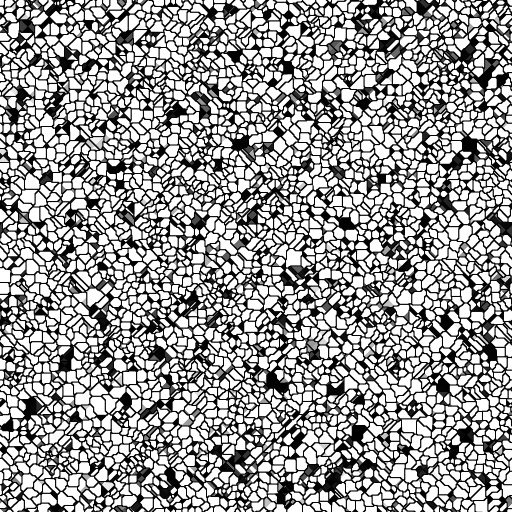
The normal is (-dU, -dV, 1) transformed by the matrix TBN. TBN = [t b n] where t is the tangent, n is the normal, and b is n * t. Now we can render images using bump mapping. The only difference between bump mapping and displacement mapping is that for the latter, we also alter fPosition and gl_Position. When calculating these values, we simply offset the position by n ∗ h(u,v) ∗ kh. Here is the texture map I used in my renders.
|
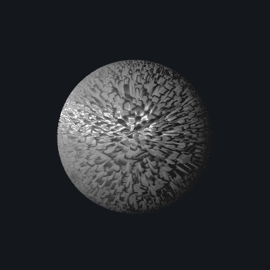
The images below show the difference between bump mapping and displacement mapping with 256 vertical and horizontal components. Bump mapping is much more subtle, while diffuse mapping creates a more drastic contrast in texture.
|
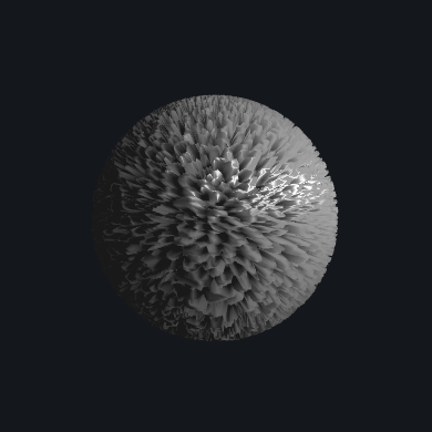
|
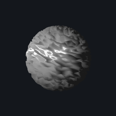
We can change the number of vertical and horizontal components to achieve different results. The images below are of the same texture map as above, but with 1024 vertical and horizontal components. The difference is not too noticable with bump mapping, but the diffuse mapping image looks quite different. The contrast in texture is even more stark, and the edges in the texture are more defined.
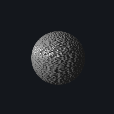
|
|
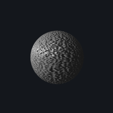
Similarly, the images below are of with the same texture map but with 64 vertical and horizontal components. The difference is much more noticable now in bump mapping, and the overall texture appears a lot smoother. With diffuse mapping, there is much less contrast and the changes in texture are more gradual.
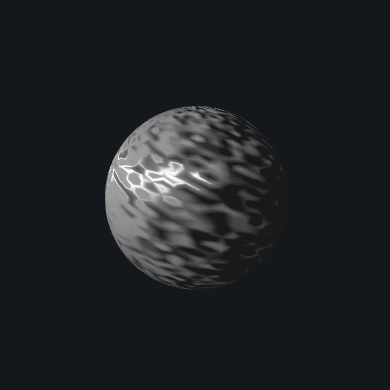
|
|
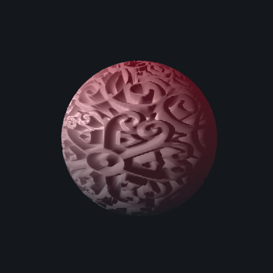
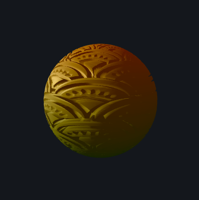
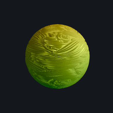
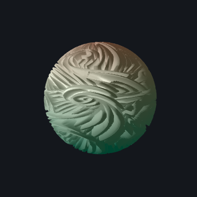
In my custom shader, I combine displacement mapping, Blinn-Phong shading, and the given extra file's color/shape changing capability. I added several new texture maps and adjusted the settings for Blinn-Phong. I then added in a variable to keep track of time and implemented color changing as in test.frag. I set this color as my ambient light. I also used the time variable to create a heartbeat-like, pulsing effect. This cannot be captured in screenshots, however. The results on different texture maps and at different points in the color cycle can be seen below.
|
|
|
|
I also implemented shaders using cube map textures. I implemented a mirror shader using reflection, and a glass shader using a combination of reflection and refraction, just as in part 1 of this project. I created a new fragment shader for each material type. I did not need to do much with vertex shaders since the geometry of the mesh is not changing. In mirror.frag, I created a new variable for the cube map texture- a samplerCube. I then calculated the incident vector as the difference between fPosition and cameraPosition and called the reflect function on the incident and normal vectors. I returned gl_FragColor as the texture of the reflected vector using the textureCube() function. In glass.frag, I defined the same values as we used in part 1- the ior, eta, and R (Schlick's coefficient). I again calculated the incident vector and the reflection vector the same way. I calculated the refraction vector as refract(incident, normal, eta). Finally, I sampled the cube map texture according to the reflection and refraction vectors, and returned the linear interpolation between them according to R. In GLSL, this can be done with the built in function mix(). The results can be seen below.
|
|