RASTERIZER

OVERVIEW

In this project, I used rasterization and several methods of sampling in order to render higher quality images while avoiding aliasing problems. Every element of this process, from the initial triangle rasterization to the final step of implementing trilinear sampling, requires precise calculations. In the final result, the difference between the various methods implemented using thse calculations can be seen in the images. There are several tradeoffs between sampling methods in terms of cost and reward, and some methods are more suited to certain images than others. Ultimately, all methods have their pros and cons, and it is very interesting to see how the process behind their implementations affects the final result.

SECTION I: RASTERIZATI0N

Part 1: Rasterizing single-color triangles

In order to rasterize a triangle, I first find the maximum x and y coordinate values among the three given points. This gives the bounding box of the triangle. Then I iterate through each point within this box and use the formula from lecture to check whether it is in the triangle or not. If the point is in the triangle, I use the fill_pixel function to fill it in. This algorithm checks each sample within the bounding box, which means it is no worse than the one described in the spec.

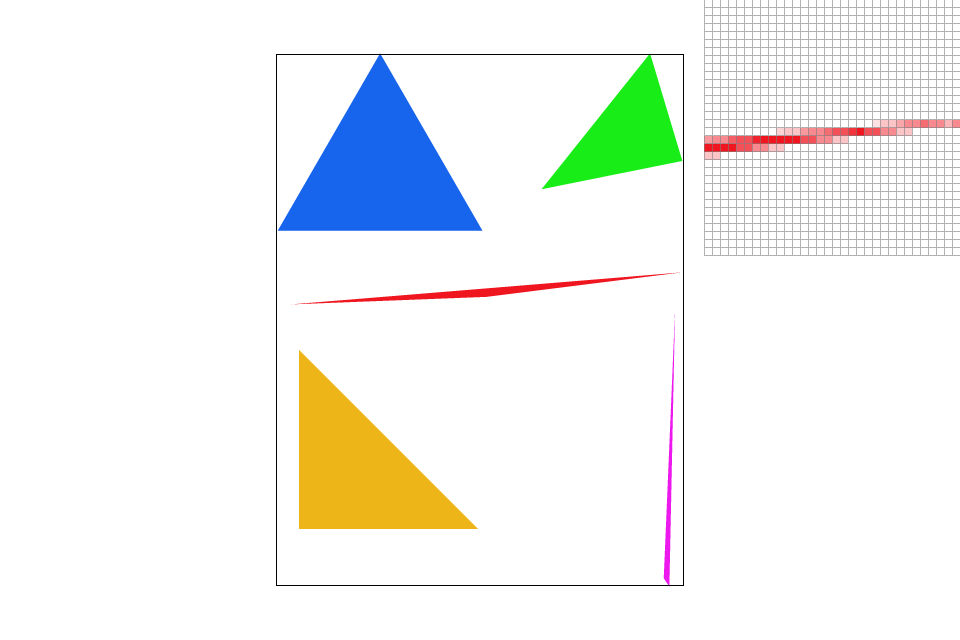
Part 2: Antialiasing triangles

The next step in the process is supersampling. To implement supersampling, I need to add two additional for loops, so I can take samples at each subpixel. I calculate the coordinates of each subpixel and then test whether or not it is in the triangle. If the point is in the triangle, I use the fill_color function to fill in that subpixel. The get_pixel_color function averages the colors of the subpixels in order to create a smoothing effect on the final image. After supersampling, the image appears much sharper and the jaggies are no longer noticable.

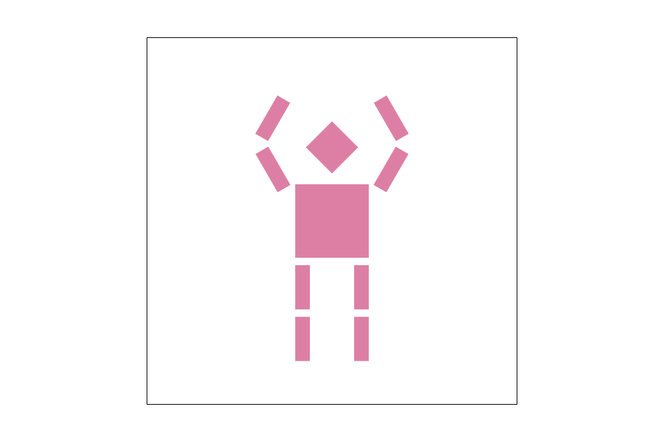
Part 3: Transforms

In this updated version of the robot.svg file, cubeman is dancing. Or maybe surrendering. Unclear. Both segments of each arm have been rotated and translated. To implement this part, I simply filled in the correct matrices for each transformation, as shown in lecture.

SECTION II: SAMPLING

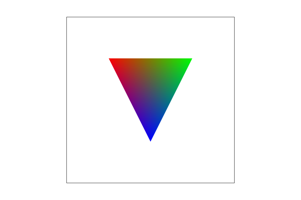
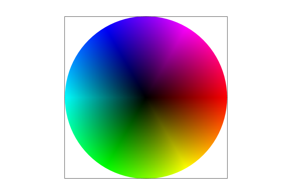
Part 4: Barycentric coordinates

Barycentric coordinates are a coordinate representation for triangles. They allow us to see the position of a point within a triangle relative to the triangle's vertices. The coordinates for a point (x, y) are (α, β, γ) such that αA + βB + γC = (x, y) and α + β + γ = 1. Each coefficient represents how close the point (x, y) is to that vertex. As the point approaches a vertex, that coefficient approaches 1. This can be represented through colors, as seen in the image of a triangle below. Points closer to the top left vertex appear more red, those closest to the top right vertex appear more green, and those closest to the bottom vertex appear more blue. Points in between are a blend of the three colors. I implemented the formula in lecture to find the barycentric coordinate representation of each point, and used their coefficient values to get the weighted color combination of each triangle. Initially I ran into a problem where the colors were not showing up probably because I hadn't multiplied them by p0_col, p1_col and p2_col. However, I debugged it and now it works perfectly.

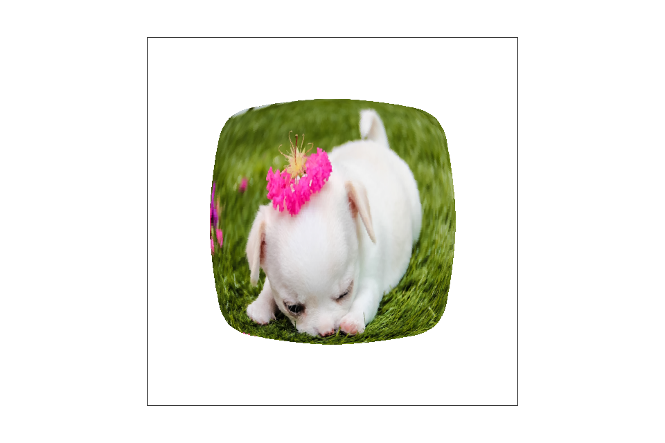
Part 5: "Pixel sampling" for texture mapping

Pixel sampling is essentially finding the texels that match up with each pixel in the final image. First I found the UV texture coordinates using the barycentric coordinates that were implememented in the previous part. The three vertex UV coordinates are interpolated using the barycentric coefficients to get the UV texture coordinate. I then retrieved the correct color from the level 0 mipmap. There are two sampling methods implemented here to do so: nearest pixel and bilinear sampling. In nearest pixel sampling, each coordinate is first scaled up by the width and height of the mipmap. I then index into the mipmap to find the rgb values associated with the correct texels. In bilinear sampling, 4 points are sampled instead of 1. I take the floor and ceiling values of each scaled x and y and sample each of the 4 generated points in the same manner as in nearest pixel sampling. I then interpolate between these colors to achieve the correct value. I initially ran into errors beause I was unsure how to properly index into the mipmap to access the texels. Eventually I saw a post on Piazza about this and was able to figure it out.

The difference between nearest pixel and bilinear can be seen in the images above. Nearest pixel clearly has more broken lines and jaggies, while bilinear sampling has a much smoother look. There will be a large difference between the two with images that include lines like the latitude/longitude ones on the globe. In lines like these the jaggies become more noticable, therefore making the image quality appear poorer.

Part 6: "Level sampling" with mipmaps for texture mapping

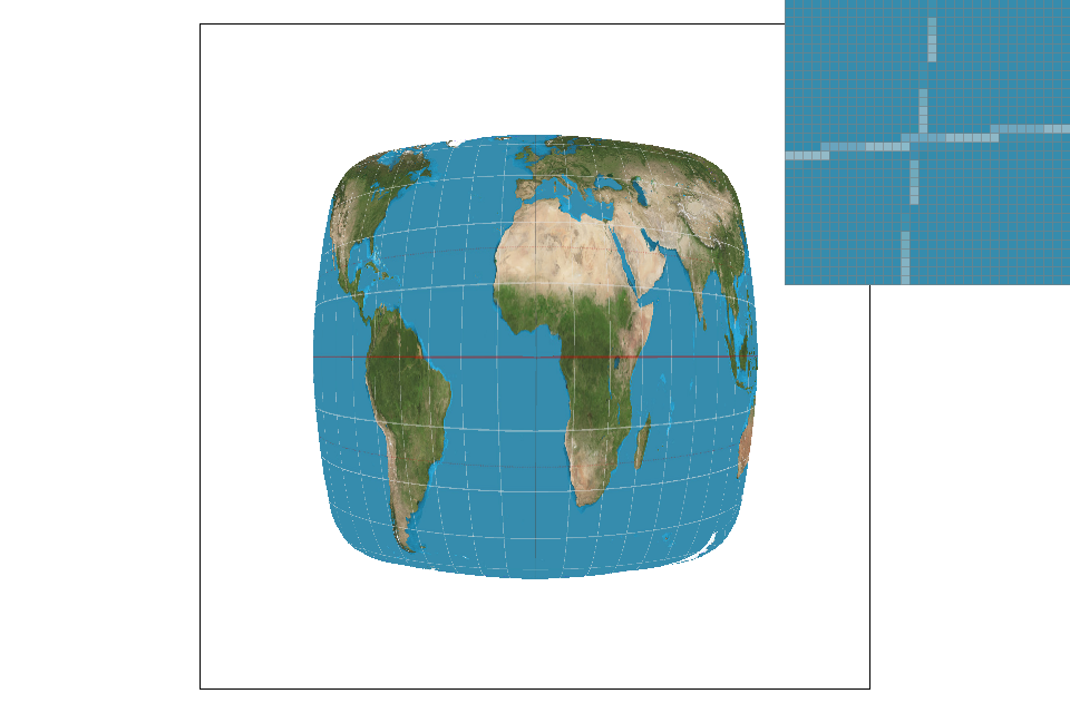
Level sampling is sampling at two adjacent mipmap levels and interpolating the results. Each mipmap level has a certain amount of pixels, and there are fewer and fewer as the level goes up. At the highest level, the image is represented as a single pixel. I first implemented the get_level function using the formula from lecture, and clamped the level values to be between 0 and the size of the mipmap. Once the level was calculated, I implemented trilinear sampling. In trilinear sampling, I took two bilinear samples at the floor and ceiling values of the current level and interpolated them. While trilinear sampling is more costly in terms of speed and memory usage, it results in less aliasing at a much lower sample rate than the other methods. Nearest pixel sampling is fastest and uses the least memory, but it has very little antialiasing power. Bilinear falls between the other two in all aspects, and therefore offers a decent balance between cost (speed and memory) and reward (antialiasing). At a higher sampling rate, the quality of the image may be better if you use bilinear of nearest pixel sampling, since trilinear sampling can result in some blurring. In my initial implementation, the image appearred significantly blurrier overall when using trilinear sampling. I was stuck on this for quite a while, but it turned out that when calculating p_dx_bary and b_dy_bary I was using the supersampling coordinates, instead of just using x and y. Once I fixed this, the image became clearer. The images below show the difference between linear interpolation using nearest pixel sampling, and full trilinear sampling. Both images are at sample rate 1, and it is clear that trilinear sampling produces far less aliasing then any other method at this sample rate.

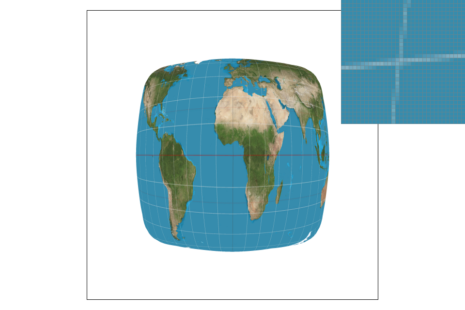
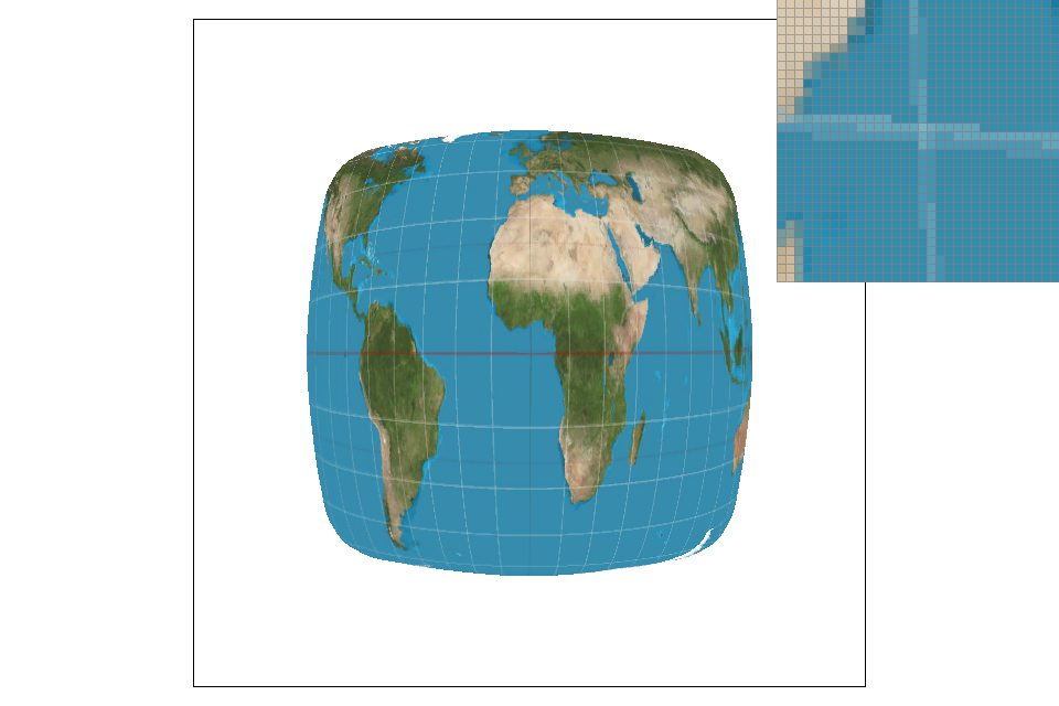
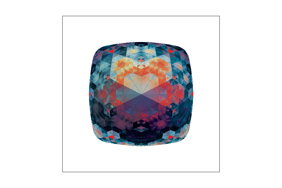
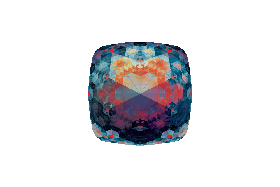
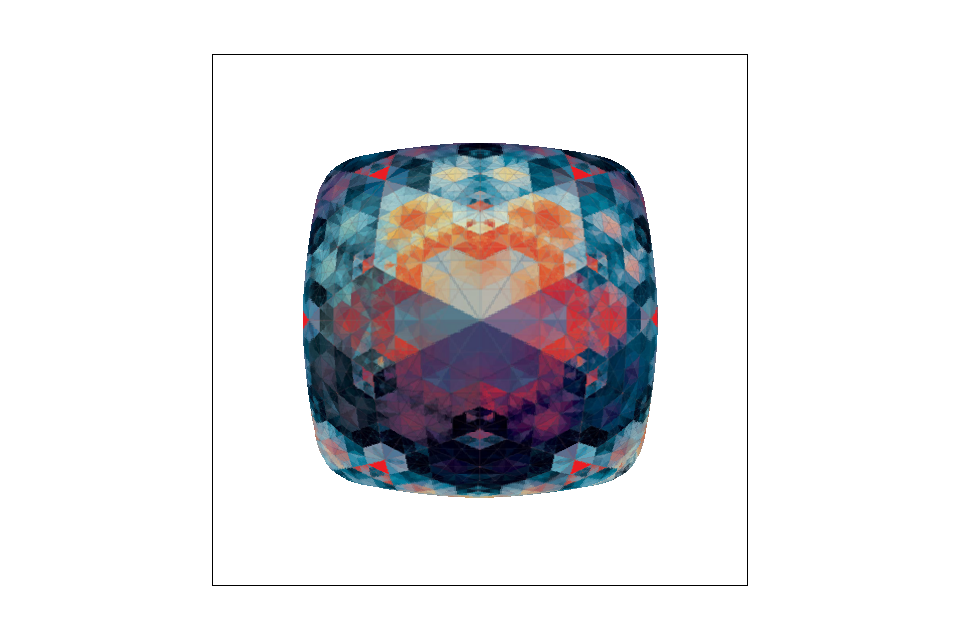
The following images demonstrate the differences between various sampling techniques.

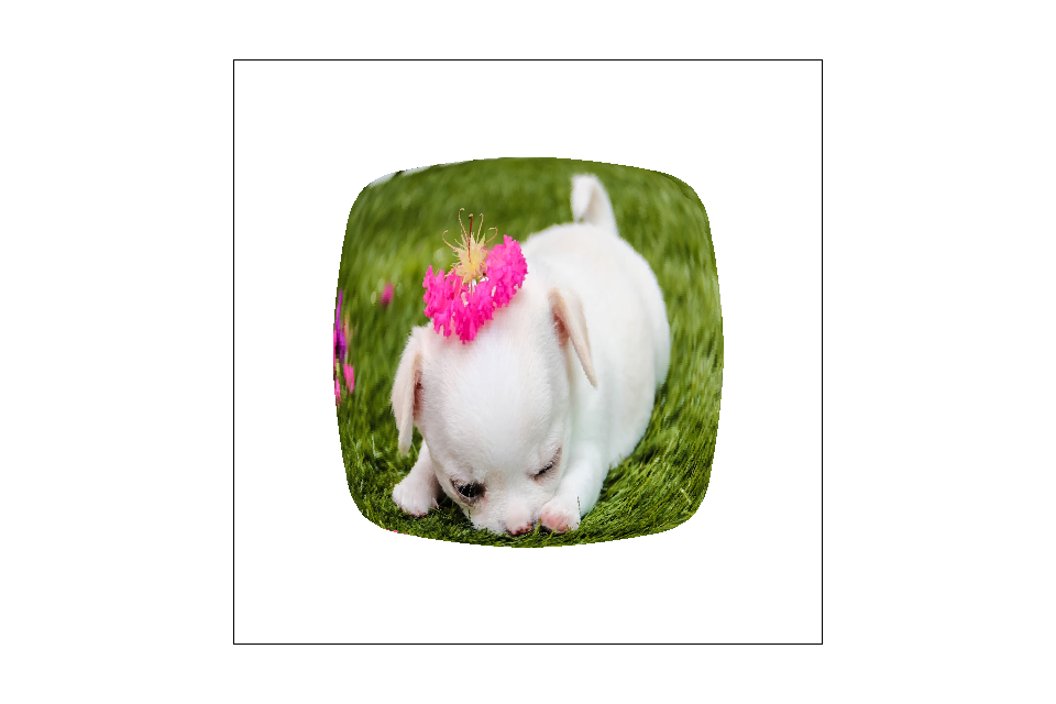
In the images above, there are no distinct lines, so the difference between the images is not as clear. They all look very similar even up close. In the images below, the difference is slightly more obvious, though not from afar. While there are certainly more jaggies when using nearest pixel sampling, the antialiasing from bilinear sampling takes away some of the contrast of the pattern, making it appear less sharp. Overall, though, from a distance the difference is not very noticable.